We can categorize longitudinal microbiome data analysis into univariate and multivariate approaches. Univariate analysis analyzes one taxon per time or first summarizes microbiome abundances into alpha diversities and then analyzes these diversities one by one. Multivariate analysis either analyzes multiple taxa simultaneously or directly tests distance/dissimilarity (beta diversities). This chapter focuses on introducing how to use the classical univariate linear mixed-effects models (LMMs) to analyze microbiome data. First, we describe linear mixed-effects models (LMMs) (Sect. 15.1), then we introduce how to implement LMMs to identify the significant taxa using the nlme package (Sect. 15.2) and model the diversity indices using the lme4 and LmerTest packages (Sect. 15.3), respectively. In Sect. 15.4, we introduce how to fit LMMs using QIIME 2. In Sect. 15.5, we provide some remarks on longitudinal microbiome studies based on LMMs. Finally, we summarize the topics of this chapter (Sect. 15.6).
15.1 Introduction to Linear Mixed-Effects Models (LMMs)
In this section, we introduce the advantages of LMMs, the development of fixed and random effects model and definition of LMMs, as well as how to conduct statistical hypothesis testing and fit LMMs.
15.1.1 Advantages and Disadvantages of LMMs
The distinctive characteristic of longitudinal study is that the subjects are measured repeatedly during the study, permitting directly assess the changes in response variable over time (Fitzmaurice et al. 2004; Diggle et al. 2002). Thus, a longitudinal study can capture between-individual differences (heterogeneity among individuals) and within-subject dynamics. Linear mixed-effects models (LMMs, aka multi-level modeling) are an important class of statistical models incorporating fixed and random effects. LMMs as a statistical method can be used to analyze correlated or non-independent data. Such data are often collected in the settings of longitudinal/repeated measurements in which the same statistical units were repeatedly measured or clustered observations where the clusters of related statistical units were measured. Such data also arise from a multilevel/hierarchical structure.
Because the circumstances of the measurements often cannot be fully controlled, considerable variation among individuals in the number and timing of observations may exist, hence resulting in unbalanced datasets. Typically, such unbalanced datasets are challenge to be analyzed using a general multivariate model with unrestricted covariance structure (Laird and Ware 1982). Moreover, missing values often arise in longitudinal/repeated measurements. Traditional statistical methods such as repeated measure analysis of variance are difficult to deal with missing values.
Mixed effects models often have advantages in dealing with unbalanced datasets and missing values.
LMMs integrate two (hierarchical) levels of observations of longitudinal data, i.e., within-group (subject) and between-group (subject) in a single model (Harville 1977; Arnau et al. 2010) and allows a variety of variance/covariance structures or correlation patterns to be explicitly modeled, which provides the opportunity to accurately capture the individual profile information over time. Typically the fixed effects are used to model the systematic mean patterns (i.e., treatment conditions), while random effects are used to model two types of random components: the correlation patterns between repeated measures within subjects or heterogeneities between subjects or both (Lee et al. 2006). That is, random effects estimate the variance of the response variable within and among these groups to reduce the probability of false positives (Type I error rates) and false negatives (Type II error rates) (Crawley 2012; Harrison et al. 2018).
In summary, the desirable features of LMMs are that they are not required for balance in the data and allow explicitly modeling and analysis of between- and within-individual variation (Laird and Ware 1982). Thus, LMMs have the capability of modeling variance and covariance (random effects) which makes this method more preferred to the classical linear model (Xia and Sun 2021). However, LMMs have the major limitation compared to the general multivariate model: a special form of the covariance structure should be assumed (Laird and Ware 1982).
15.1.2 Fixed and Random Effects
The core feature of LMMs is that they incorporate fixed and random effects and hence can analyze the fixed and random effects simultaneously. A fixed effect refers to a parameter that does not vary, whereas a random effect represents a parameter that is itself a random variable. In other words, the distribution of these parameters (or “random effects”) vary over individuals (Laird and Ware 1982).
LMMs have a long history of development. In 1918 Ronald Fisher introduced the random effects models to study the correlations of trait values between relatives such as the correlation of parent and child (Fisher 1918; Laird and Ware 1982). Since the 1930s, researchers have emphasized taking account of random effects as accurately as possible when estimating experimental treatment effects (fixed effects) (Thompson 2008). In the 1950s, Charles Roy Henderson provided best linear unbiased estimates (BLUE) of fixed effects and best linear unbiased predictions (BLUP) of random effects (Robinson 1991; Henderson et al. 1959; McLean et al. 1991). Subsequently, Goldberger (1962), Henderson (Henderson 1963, 1973, 1984; Henderson et al. 1959), and Harville (1976a, b) developed mixed model procedures. The mixed model equations (Henderson 1950; Henderson et al. 1959) introduced by Charles Roy Henderson offers the base for a methodology that provides flexibility of fitting models with various fixed and random elements with the possible assumption of correlation among random effects (McLean et al. 1991; Thompson 2008).
15.1.3 Definition of LMMs
In matrix form a linear mixed model can be specified as:

G is the variance-covariance matrix of the random effects. Given the fixed effects are directly estimated, the random effects are just deviations around the value in β, which is the mean. Thus it the variance that is left to estimate. Various structures of the variance-covariance matrix of the random effects can be assumed and specified. If only a random intercept is specified, then G is just a 1 × 1 matrix, which models the variance of the random intercept. If a random intercept and a random slope are assumed, then we can specify:
![$$ G=\left[\begin{array}{cc}{\sigma}_{\mathrm{int}}^2& {\sigma}_{\operatorname{int},\mathrm{slope}}^2\\ {}{\sigma}_{\operatorname{int},\mathrm{slope}}^2& {\sigma}_{\mathrm{slope}}^2\end{array}\right] $$](images/486056_1_En_15_Chapter_TeX_IEq1.png) . If we assume that the random effects are independent, then the true structure is
. If we assume that the random effects are independent, then the true structure is ![$$ G=\left[\begin{array}{cc}{\sigma}_{\mathrm{int}}^2& 0\\ {}0& {\sigma}_{\mathrm{slope}}^2\end{array}\right] $$](images/486056_1_En_15_Chapter_TeX_IEq2.png) . In Chap. 16 (Sect. 16.2), we will introduce generalized linear mixed models (GLMMs).
. In Chap. 16 (Sect. 16.2), we will introduce generalized linear mixed models (GLMMs).
15.1.4 Statistical Hypothesis Tests
In the statistical model building for experimental or observational data, LMMs can be used to serve two purposes (Bates 2005): (1) to characterize the dependence of a response (outcome variable) on covariate(s), conditioning on the treatment status and the time under treatment, and (2) to characterize the “unexplained” variation in the response.
A mixed-effects model (or more simply a mixed model) incorporates both fixed-effects terms and random-effects terms, which use a different way to model repeatable covariates and non-repeatable covariates (Bates 2005; Bates et al. 2015). The fixed-effects terms are used for a repeatable covariate to characterize the change in the response between different levels such as typically the change of the response over time under treatment or the difference of a response between treatment and the control groups. In contrast, the random-effects terms are used to characterize the variation induced in the response by the different levels of the non-repeatable covariate (a grouping factor).

The LRT statistic for the test of the hypothesis is given:

 is a subspace of the parameter space Θβ of the fixed effects β. The log-likelihood ratio test statistic for the null hypothesisis is given by:

We will describe more details about the LRT and other tests in Chap. 16 (Sect. 16.5.4 for the LRT).
15.1.5 How to Fit LMMs
First of all, exactly determining whether a variable is a random or fixed is controversial.
Specifying a particular variable as fixed or random effect or even both simultaneously largely depends on experimental design and context. Generally fixed effects refer to all factors whose levels are experimentally determined or whose interest is in the specific effects of each level, such as treatments, time, other covariates, as well as treatment and time (or covariates) interactions. In contrast, random effects refer to all factors that qualify as sampling from a population or whose interest is in the variation among the population rather than the specific effects of each level. Random effects typically represent some grouping variables in both subject and unit levels (Breslow and Clayton 1993), such as individuals in repeated measurements, field trials, plots, blocks, batches.
- 1.
Fitting random effects requires at least five “levels” (groups) for a random intercept term to achieve robust estimates of variance (Gelman and Hill 2007; Harrison 2015). The mixed model may not be able to estimate the among-group variance accurately for less than 5 levels (Harrison et al. (2018) because if the random effect models have less than 5 levels, then the variance estimate will either collapse to zero, making the model become an ordinary GLM (Gelman and Hill 2007) or be non-zero which is incorrect if the small number of groups that were sampled are not representative of true distribution of means (Harrison 2015). Thus, in practice, as a rule of thumb, the factors with fewer than 5 levels are considered as fixed effects, while the factors with numerous levels are considered as random effects in order to increase accurately estimating variance.
- 2.
Models and especially the random slope models will be unstable if sample sizes across groups are highly unbalanced (Grueber et al. 2011).
- 3.
It is difficult to determine the significance or importance of variance among groups.
- 4.
Mis-specification of random effects or incorrectly parameterizing the random effects in the model could results in the model estimates being unreliable as ignoring the need for random effects altogether (Harrison et al. 2018).
Second, start with a full model to include all potential independent variables in the fixed model using maximum likelihood (ML).
Third, fit the random model using restricted maximum likelihood (REML) to optimize the random structure.
Finally, refit the optimal fixed and random models using REML, and validate and interpret the modeling results.
After updating (refitting) optimal model with REML, we can check the differences in the main effects and effects in interaction terms caused by the introduction of random effects. A diagnosing model fit procedure can be conducted to validate the fitted models. The reader is referred to Chap. 17 for details. We then can interpret the results based on the prior hypotheses.
15.2 Identifying the Significant Taxa Using the nlme Package
In this section, we introduce LMMs in microbiome research and illustrate how to fit LMMs to identify significant microbial taxa.
15.2.1 Introduction to LMMs in Microbiome Research
The microbiome is inherently dynamic, driven by interactions with the host and the environment, and varies over time. Longitudinal microbiome data analysis can enhance our understanding of short- and long-term trends of microbiome by intervention, such as diet, and the development and persistence of chronic diseases caused by microbiome. Thus, longitudinal microbiome data analysis provides rich information on the profile of microbiome with host and environment interactions (Xia et al. 2018a).
In the literatures of longitudinal statistical analysis of physical, biological, psychological, social, and behavioral sciences, the linear mixed-effects models (LMMs) (Laird and Ware 1982) are often used. The classical LMM method was also one of the first models that were used to analyze longitudinal microbiome data (e.g., Rosa et al. 2014; Kostic et al. 2015; DiGiulio et al. 2015; Wang et al. 2015) and currently is still used in microbiome and multi-omics literature (Lloyd-Price et al. 2019). The reasons that LMMs have been chosen to analyze longitudinal microbiome data mainly because (1) LMMs equip with fixed- and random-effects components, which provides a standardized and flexible approach to model both fixed- and random-effects. (2) LMMs can jointly model measures over all the time points to account for time-dependent correlations in longitudinal microbiome study designs. Specifically because (3) LMM method was an established methodology to remove the effects of fixed- and random-effect confounding variables (Ernest et al. 2012; Xia 2020) in the areas of microarray, genome-wide association studies (GWAS), and metabolomics (Fabregat-Traver et al. 2014; Zhao et al. 2019), which motivates its application to microbiome data.
15.2.2 Longitudinal Microbiome Data Structure
Microbiome data (i.e., OTUs/ASVs table) generated by each sample through either the 16S rRNA gene sequencing or the shotgun metagenomics sequencing consist of read counts of taxa at certain taxonomic levels, such as kingdom, phylum, class, order, family, genus, and species. In longitudinal microbiome study, each subject are measured at multiple time points (i.e., samples). Assume that there are n subjects, and subject i is measured at ni time points tij, j = 1, …, ni and i = 1, …, n. Denote Cijm as read counts for subject i measured at time j for taxon m, m = 1, …, m, and denote the total sequence read counts for subject i at time j as Tij, which is referred to as library size or depths of coverage; then a longitudinal microbiome data structure can be summarized in Table 15.1.
Longitudinal microbiome data structure
Subject-ID | Taxon 1 | Taxon 2 | ⋯ | Taxon m | Total reads | Covariate | Time |
|---|---|---|---|---|---|---|---|
Subject 1 | C111 | C112 | … | C11m | T11 | X1 | t11 |
Subject 1 | C121 | C122 | … | C12m | T12 | X1 | t12 |
Subject 1 | C131 | C132 | … | C13m | T13 | X1 | t13 |
Subject 2 | C211 | C212 | … | C21m | T21 | X2 | t21 |
Subject 2 | C221 | C222 | … | C22m | T22 | X2 | t22 |
Subject 2 | C231 | C232 | … | C23m | T23 | X2 | t23 |
⋮ | ⋮ | ⋮ | ⋮ | ⋮ | ⋮ | ⋮ | ⋮ |
Subject n | Cn11 | Cn12 | … | Cn1m | Tn1 | Xn | Tn1 |
To analyze the associations between the microbiome and the host trait of interest (i.e., covariate variables), two approaches can be applied via LMMs: (1) fit LMMs using the read counts as the outcome and (2) fit LMMs using the diversity index as the outcome. The LMMs can be fitted using the nlme (current version 3.1-157, March 2022) and lme4 (current version 1.1-29, April 2022) packages. Below we illustrate their uses through our dataset of breast cancer QTRT1 mouse gut microbiome.
15.2.3 Fit LMMs Using the Read Counts as the Outcome
When applying LMM to fit microbiome and multi-omics abundance data, raw microbiome abundances should be transformed or normalized by an appropriate method (Xia 2020): (1) arcsine square root transformation (Kostic et al. 2015; Rosa et al. 2014), (2) log-transformation (with pseudocount 1 for zero values) (Lloyd-Price et al. 2019), and (3) log-transformation with no pseudocount for expression ratios (non-finite values removed) (Lloyd-Price et al. 2019).
It is arguable whether or not these transformation/normalization methods are appropriate to each outcomes of interest. Especially adding a pseudocount 1 for zero values may even not make sense because it forces the microbiomes from “nothing” (absence) to “being”(presence).
In this dataset, the mouse fecal samples were collected at two time points: pretreatment and posttreatment. Below we use LMMs to identify the significant change species over time.
Step 1: Load taxa abundance data and meta data.
Step 2: Check taxa and meta data.
Step 3: Create analysis dataset-outcomes and covariates.
There are 59 taxa in otu_tab. To effectively model the outcomes, we first reduce the number of taxa in the analysis.
In the literature, there are no unique procedures to filter abundance taxa data before modeling. In general, the unclassified taxa were removed, then either read counts or relative abundance data were used. Some researchers renormalized the data after the unclassified taxa were removed, while others directly used the data but adjusted the total read counts during the modeling. Some researchers consider low read counts contribute less to outcome results (although this argument underestimates the functional analysis or the role of rare taxa) and hence removed the low read counts based on a cutoff value. Because too few zeros and too many zeros in the abundance data may cause the models be inaccurate, most models used the proportion of zeros to filter abundance taxa data. Some even used double functions (sum() and quantile() functions) (Xia et al. 2018b) to filter the data. Actually, such arbitrary data preprocessing is an unapproved practice in microbiome research. We should recognize that it is a limitation of current microbiome research.
Here, we use sum() and quantile() functions to double filter the taxa that results in 17 taxa to be included in the analysis.
If the meta data are incomplete, we can use the complete.cases() function to subset the data and apply complete cases.
Step 4: Run the lme() function in the nlme package to implement LMMs.
The lme () function is available in the R package nlme, which was developed to fit linear mixed models of the form described in Pinheiro and Bates (2000) (Pinheiro and Bates 2000, 2006).
We can assume independence of correlation matrix by setting R matrix as an identity matrix, which is the most simplified structure. However, various correlation matrices can be specified (Pinheiro and Bates 2000, 2006) such as autoregressive of order 1 [AR(1)] or continuous-time AR(1). The lme () function allows for multiple and correlated group-specific (random) effects (the argument random) and various types of within-group correlation structures (the argument correlation) described by corStruct in the nlme package.
Below we fit LMMs with main host factors: group and time as well as their interaction as fixed effects and random intercept only (Group*Time, random = ~ 1|Subject). Other LMMs also can be fitted such as with main host factors: group, time, and their interaction as fixed effects and random intercept only and specifying correlation matrix (Group*Time, random = ~ 1|Subject, correlation = corAR1()).
First we need to create list() and matrix to hold the objects of modeling results, which could be used as further processing the results and model comparisons. Then we need to call library(nlme) and run the lme() function iteratively to fit multiple taxa (outcome variables).
Step 5: Adjust P-values.
Step 6: Write table to contain the results (Table 15.2).
Modeling results from linear mixed effects model based on QtRNA data
taxa_all | Group_Imm_adj | TimePost_Imm_adj | Group.TimePost_Imm_adj | |
|---|---|---|---|---|
1 | D_6__Anaerotruncus sp. G3(2012) | 0.5954 | 2E-04 | 0.8432 |
2 | D_6__Clostridiales bacterium CIEAF 012 | 0.9589 | 0.6811 | 0.4371 |
3 | D_6__Clostridiales bacterium CIEAF 015 | 0.4575 | 2E-04 | 0.3968 |
4 | D_6__Clostridiales bacterium CIEAF 020 | 0.3038 | 0.1708 | 0.1857 |
5 | D_6__Clostridiales bacterium VE202-09 | 0.9589 | 0.2281 | 0.4862 |
6 | D_6__Clostridium sp. ASF502 | 0.8211 | 0.3766 | 0.5562 |
7 | D_6__Enterorhabdus muris | 0.1482 | 0.8121 | 0.3488 |
8 | D_6__Eubacterium sp. 14-2 | 0.0654 | 6E-04 | 0.1857 |
9 | D_6__gut metagenome | 0.8211 | 0.8808 | 0.5562 |
10 | D_6__Lachnospiraceae bacterium A4 | 0.8309 | 0.6208 | 0.4494 |
11 | D_6__Lachnospiraceae bacterium COE1 | 0.1329 | 0.4969 | 0.0277 |
12 | D_6__mouse gut metagenome | 0.4186 | 3E-04 | 0.8432 |
13 | D_6__Mucispirillum schaedleri ASF457 | 0.0644 | 0.7033 | 0.1857 |
14 | D_6__Parabacteroides goldsteinii CL02T12C30 | 0.353 | 0.0026 | 0.9993 |
15 | D_6__Ruminiclostridium sp. KB18 | 0.8211 | 0.0026 | 0.1857 |
16 | D_6__Staphylococcus sp. UAsDu23 | 0.1482 | 6E-04 | 0.3249 |
17 | D_6__Streptococcus danieliae | 0.9589 | 0.4471 | 0.8743 |
15.3 Modeling the Diversity Indices Using the lme4 and LmerTest Packages
In this section, we introduce the lme4 and lmerTest packages and illustrate how to fit LMMs to analyze the diversity indices.
15.3.1 Introduction to the lme4 and lmerTest Packages
The lme4 package (Bates 2005; Bates et al. 2015) and its lmer() function were developed by Bates and his colleagues to provide more flexible fitting of linear mixed models and provide extensions to generalized linear mixed models as well. Compared to the lme () function, the lmer() function fits a larger range of models and is more reliable and faster, but the model specification has been changed slightly. For the details on how to use the lmer() function to fit linear mixed models, and the differences between lmer() and lme(), the interested reader is referred to the cited references for description of the methods (Bates 2005; Bates et al. 2015).
Obtain the P-values for the F-and t-tests for objects returned by the lmer() through overloading the anova() and summary() functions of fixed effects.
Implement the Satterthwaite’s method for approximating degrees of freedom for the t-and F-tests.
Implement the construction of Type I-III ANOVA tables.
Obtain the summary and the anova table using the Kenward-Roger approximation for denominator degrees of freedom by using the KRmodcomp() function in the pbkrtest package.
Perform backward elimination (a step-down model building method) of both random and fixed non-significant effects.
Calculate population means and perform multiple comparison tests as well as plot facilities.
The lme4 package provides F-statistics and the t-statistics in anova() and summary() functions, respectively; however, the P-values for the corresponding F- and t-tests are not provided. The lmerTest package implements and wraps Satterthwaite’s method (Giesbrecht and Burns 1985; Hrong-Tai Fai and Cornelius 1996) into anova() and summary() functions for the object returned by lmer(). Satterthwaite’s method has been implemented in SAS software (SAS Institute Inc. 1978, 2013). The SAS users should be familiar with Satterthwaite’s method. As an alternative, the Kenward-Roger approximation method is also available, which is integrated through the KRmodcomp() function of the pbkrtest package (Halekoh and Højsgaard 2014, 2021). For details, the interested reader is referred to the paper of lmerTest package (Kuznetsova et al. 2017).
15.3.2 Fit LMMs Using the Diversity Index as the Outcome
In this subsection, we use the same dataset from Example 15.1 to assess the association between microbiome diversity and group status (Genotype) by setting the Chao 1 richness index as the outcome and the group and time as the fixed-effect terms.
We fit the LMMs using the R package lme4 (Bates et al. 2015) and perform the corresponding statistical test using the R package lmerTest (Kuznetsova et al. 2017).
For illustration, we select the Chao 1 richness index as the response variable and the group, time, and their interaction as the fixed-effect terms. We also consider group and group by time interaction as random terms. We use the following five steps to perform LMMs and illustrate the functionality of lme4 and LmerTest packages.
Step 1: Load taxa abundance data and meta data.
Step 2: Calculate alpha-diversity indices.
Here we choose Chao 1 richness index as response variable. Similarly, other diversity indices can be applied. Below we use the ampvis2 package to calculate Chao 1 richness index. It can be calculated using other R packages such as vegan and microbiome packages.
Step 3: Run LMMs using the ANOVA method for objects returned by lmer() function.
The lmerTest package provides Type I, II, and III ANOVA tables as defined in the SAS software (SAS Institute Inc. 1978). The Type II and III tables do not depend on the order in which the effects are entered in the model, whereas the Type I ANOVA table is order dependent which performs the sequential decomposition of the contributions of the fixed-effects. The Type I table is the one produced by the ANOVA method of the lme4 package (Bates et al. 2015; Kuznetsova et al. 2017).
The columns DenDF and Pr(>F) refer to denominator degrees of freedom and P-values, which are calculated using the Satterthwaite’s method of approximation. Based on the P-values, the Chao 1 richness index for Group and Time interaction is marginally significant (P = 0.077).
The Time variable is statistically significant (P = 0.0037) and the Group by Time interaction is marginally statistically significant (P = 0.0775) from the Type I ANOVA table with Satterthwaite’s approximation.
We can require another type of ANOVA by changing the type argument and Kenward-Roger’s method for calculating the F-test. The following commands require the Type I ANOVA table with Kenward-Roger’s approximation.
Step 4: Run LMMs using the summary method for objects returned by the lmer() function.
REML criterion at convergence: 348.2
In the output, additional columns of df and Pr(>|t|) in the fixed effects are added to the lme4 package. The df refers to degrees of freedom based on Satterthwaite’s approximation and Pr(>|t|) is the P-value for the t-test with df as degrees of freedom.
Step 5: Perform backward elimination using the step method for objects returned by the lmer() function.
To illustrate the step method for backward elimination, here we consider a full model including Group, Time, and their interaction as fixed-effect terms, as well as Group and Group by Time interaction as random-effect terms.
Backward reduced random-effect table:
The reduced model showed that Group and Time interaction in fixed-effect terms is marginally significant (P = 0.0775) and Time is significant (P = 0.0045).
15.4 Implement LMMs Using QIIME 2
In Chap. 9 (Sect. 9.5.4), we used this study to illustrate how to obtain core alpha diversities via QIIME 2 and then we used pairwise Kruskal-Wallis test to compare Sex by Time variables interaction. There are total 349 samples (208 for early and 141 for late times). The results showed that later time has larger Shannon diversity than early time with P-value of 0.003227 and Q-value of 0.003227. In Chap. 9, we commented that Kruskal-Wallis test does not consider the dependency of the individuals/subjects and a longitudinal model is more appropriate. Here we use QIIME 2 to implement LMMs to test whether Shannon diversity index changed over time and had gender difference in this study.
15.4.1 Introduction to the QIIME Longitudinal Linear-Mixed-Effects Command
Linear mixed-effects models (LMMs) are more flexible in modeling the association between a single response variable and one or more independent variables in a longitudinal or repeated-measures design. The qiime longitudinal linear mixed-effects perform LMMs to evaluate the covariates effects of “group_columns” and “random_effects” to a single dependent variable (“metric”) and plot line plots of each group column. To implement LMMs, at least one numeric state-column (e.g., time variable) and one or more comma-separated group-columns need to be specified as the fixed effects, i.e., independent variables. These fixed effects may be categorical or numeric metadata columns. After implementing this model, regression plots of the response variable (“metric”) are plotted as a function of the state column and each group column.
15.4.2 Fit LMMs in QIIME 2
First, we need activate QIIME 2. Open the terminal and type: source activate qiime2-2022.2, which is latest version of QIIME 2. When the terminal appears “(qiime2-2022.2),” it indicates qiime2-2022.2 version has been activated. We can work with this version now.
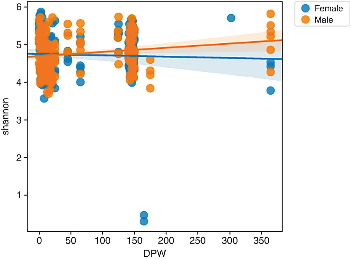
A scatterplot of Shannon versus D P W plots female and male. An increasing line and an almost horizontal line mark the trend of male and female, respectively.
Regression scatterplots of Shannon diversity by male and female mice
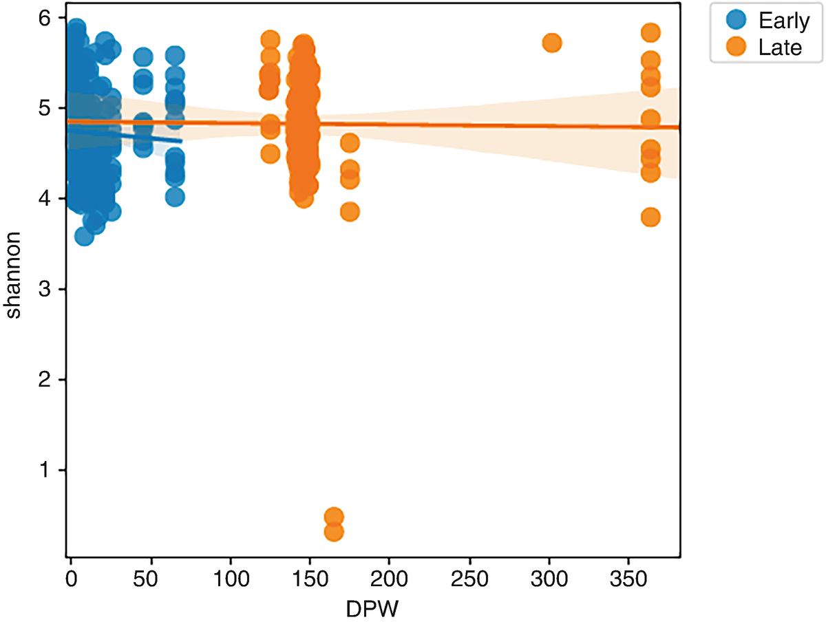
A scatterplot of Shannon versus D P W plots early and late. A decreasing line from (0, 4.9) to (375, 4.8) marks the trend of late, and a decreasing line from (0,4.8) to (55,4.7) marks the trend of early. Values are approximated.
Regression scatterplots of Shannon diversity by early and later times

A text reads, saved visualization to, L M M E f f e c t s M i S e q underscore S O P dot q z v.
where the four columns are required: (1) sample metadata (here, SampleMetadataMiSeq_SOP.tsv) which contains individual-id-column; (2) state-column parameter: metadata column containing state (time) variable (here, DPW); (3) individual-id-column parameter, metadata column containing study IDs for individual subjects (here, StudyID), which indicates the individual subject/site that was sampled repeatedly; and (4) the o-visualization output column.
The p-metric is used to specify the response (dependent) variable column name, which must be located in the metadata or feature table files if the feature table is provided as input data. The p-group columns is used to specify the metadata columns as the independent covariates that are used to determine mean structure of “metric.” Several fixed-effects variables can be specified via a comma-separated list. The p-random-effects parameter can be added. The random-effects metadata columns are used to specify the independent covariates that are used to determine the variance and covariance structure (random effects) of “metric.” A random intercept for each individual is set by default, while to specify a random slope, set the variable in the p-state-column, in which the state-column value is passed as input to the random-effects parameter. Same to fixed effects, to specify several random effects, a comma-separated list of random effects can be provided in the p-random-effects column. The o-visualization output is used to name VISUALIZATION outputs. We here named it as LMMEffectsMiSeq_SOP.qzv.
By reviewing LMMEffectsMiSeq_SOP.qzv via qiime2 view, we can see that there were no statistically significant effects of sex (P = 0.088) or sampling period (early vs. late, P = 0.356) on Shannon diversity index, which confirmed the results that were originally reported in Schloss et al. (2012).
The qiime longitudinal linear-mixed-effects command returns several results, including (1) the input parameters at the top of the visualization, (2) the Model summary of descriptive information about the LMMs, (3) the main Model results, which summarizes the effects of each fixed effect (and their interactions) on the dependent variable (here, Shannon diversity). This table shows parameter estimates, including standard errors, z scores, P-values (P>|z|), and 95% confidence interval upper and lower bounds for each parameter, (4) the Regression scatterplots that categorized by each “group column” at the bottom of the visualization, with linear regression lines and 95% confidence interval in gray for each group, and (5) Projected Residuals, the scatterplots of fit vs. residual plots. The plots show the relationship between metric predictions for each sample (on the x-axis), and the residual or observation error (prediction - actual value) for each sample (on the y-axis). They are used for diagnostics. The roughly zero-centered residuals suggest a well-fitted model.
Below we add random-effects parameters and specify DPW as a random effect. For details of how specifying random effects, the reader is referred to Sect. 15.1.5 How to Fit LMMs.

A text reads, saved visualization to, L M M E f f e c t s M i S e q underscore S O P underscore R a n d o m dot q z v.
The above regression scatterplots in Figs. 15.1 and 15.2 just provide a quick summary information of the data. To interactively plot the longitudinal data, QIIME 2 recommends using the volatility plot.
15.4.3 Perform Volatility Analysis
Volatility analysis generates interactive line plots to visualize how a dependent variable is volatile over a continuous, independent variable (e.g., time) in group(s). Thus, a volatility plot is a good qualitative tool to identify outliers that disproportionately drive the variance within individuals and groups.
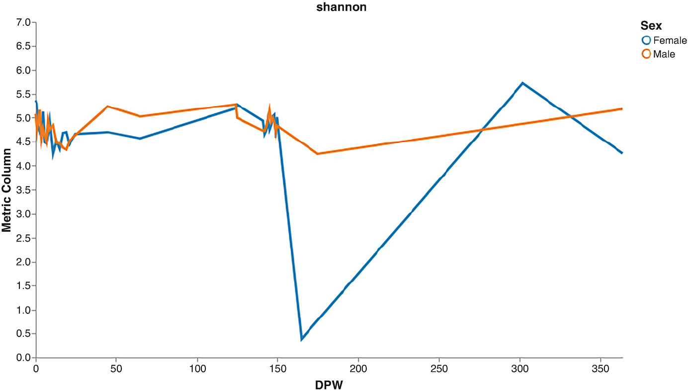
A line graph of metric column versus D P W plots lines for the female and male. The female line starts at (0, 5.4), fluctuates and drops to (160, 0.4), raises to (290, 5.7), and again drops. The male line starts at (0, 5.2), fluctuates, and ends at (375, 5.5). Values are approximated.
Volatility plots of Shannon diversity by male and female mice

A text reads, saved visualization to, V o l a t i l i t y S e x L M M E f f e c t s M i S e q underscore S O P dot q z v.
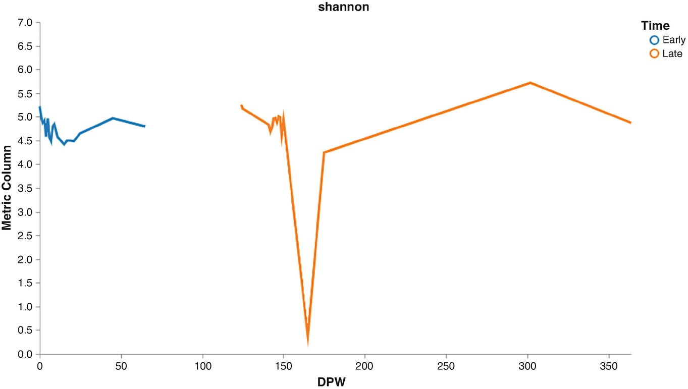
A line graph of metric column versus D P W plots lines for early and late. The early line starts at (0, 5.3), fluctuates, and ends at (55, 4.8). The late line starts at (125, 5.3), drops to (160, 0.2), raises, and then decreases. All values are approximated.
Volatility plots of Shannon diversities by early and later times

A text reads, saved visualization to, V o l a t i l i t y T i m e L M M E f f e c t s M i S e q underscore S O P dot q z v.
By reviewing the resulted output visualization using QIIME 2 view, the plot displays a line plot on the left-hand side of and a panel of “Plot Controls” to the right-hand side.
The “Plot Controls” panel is used to interactively adjust variables and parameters for determining how “groups” and “individuals” values change across the specified state-column (a single independent variable). For details on how use the interactive features, the reader is referred to QIIME 2 documents for further references or practicing the output visualization in QIIME 2 view.
15.5 Remarks on LMMs
The development of new methods for analysis of microbiome data often takes the advantage of LMM framework such as in Zhang and Yi (2020) and Hui et al. (2017). However, LMM is not specifically designed for microbiome data, and hence it does not address issues due to characteristics of microbiome data. LMM method is often criticized for using to analyze microbiome data because (1) it needs to transform absolute abundance read account into the relative abundance via a transformation method (e.g., arcsine square root transformation) before fitting the model, and most often treats transformed microbiome abundance as normally distributed responses (such as in Srinivas et al. 2013; Rosa et al. 2014; Leamy et al. 2014; Wang et al. 2015); (2) it does not explicitly handle the excess zeros in the data (Chen and Li 2016), and thus cannot fit the model with zero-inflation and over-dispersion to address the sparsity issue (Zhang and Yi 2020). Thus, directly applying LMM method to analyze microbiome data may be underpowered and have potential bias to identify the dynamic microbiome effects.
Several proposed longitudinal microbiome models have compared their methods to LMM method (Chen and Li 2016; Zhang et al. 2018; Zhang and Yi 2020).
15.6 Summary
This chapter focused on LMMs to microbiome data analysis. Section 15.1 covered the general topics of LMMs including the advantages and disadvantages of using LMMs, definitions of fixed and random effects, and its formulation, statistical hypothesis testing, and the procedures of fitting LMMs. Section 15.2 described how to identify the significant taxa with the nlme package. A general introduction to LMMs in microbiome research and longitudinal microbiome data structure were also described. Section 15.3 introduced the lme4 and LmerTest packages and how to use these two packages to analyze the diversity indices. Section 15.4 described how to implement LMMs in QIIME 2, including introduction to the QIIME longitudinal linear-mixed-effects command and volatility analysis. Section 15.5 provided some general remarks on LMMs in microbiome data.
Chapter 16 will describe the generalized linear mixed models (GLMMs), and Chap. 17 will introduce GLMMs and zero-inflated GLMMs for longitudinal microbiome data.